Bernoulli Distribution

Bernoulli Distribution:

Definition: The Bernoulli Distribution is a discrete probability distribution that models a random experiment with two possible outcomes - success (usually denoted as 1) and failure (usually denoted as 0). It is named after Swiss mathematician Jacob Bernoulli.
Probability Mass Function (PMF): The PMF of the Bernoulli Distribution is defined as:
${\begin{cases}q=1-p&{\text{if }}k=0\\p&{\text{if }}k=1\end{cases}}$
Mean and Variance: The mean (expected value) of the Bernoulli Distribution is $p$ , and the variance is $p (1 - p)$ .

Mean
The expected value of a Bernoulli random variable $X$ is
$\operatorname {E} [X]=p$
This is due to the fact that for a Bernoulli distributed random variable $X$ with $\Pr(X=1)=p$ and $\Pr(X=0)=q$ we find
$\operatorname {E} [X]=\Pr(X=1)\cdot 1+\Pr(X=0)\cdot 0=p\cdot 1+q\cdot 0=p.$
Variance
The variance of a Bernoulli distributed $X$ is
$\operatorname {Var} [X]=pq=p(1-p)$
We first find
$\operatorname {E} [X^{2}]=\Pr(X=1)\cdot 1^{2}+\Pr(X=0)\cdot 0^{2}=p\cdot 1^{2}+q\cdot 0^{2}=p=\operatorname {E} [X]$
From this follows
$\operatorname {Var} [X]=\operatorname {E} [X^{2}]-\operatorname {E} [X]^{2}=\operatorname {E} [X]-\operatorname {E} [X]^{2}=p-p^{2}=p(1-p)=pq$ ^[2]
With this result it is easy to prove that, for any Bernoulli distribution, its variance will have a value inside $[0,1/4]$ .

Graphical Representation:
Here's a bar graph illustrating the Bernoulli Distribution for different values of $p$ :

Bernoulli distribution
Probability mass function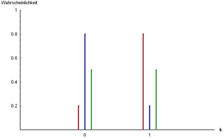
Three examples of Bernoulli distribution:
   $P(x=0)=0{.}2$ and $P(x=1)=0{.}8$
   $P(x=0)=0{.}8$ and $P(x=1)=0{.}2$
   $P(x=0)=0{.}5$ and $P(x=1)=0{.}5$

In this graph, you can see that the probability of success ( $p$ ) is represented by the height of the bar at $x = 1$ , and the probability of failure ( $1 - p$ ) is represented by the height of the bar at $x = 0$ . Since it's a discrete distribution, there are only two possible outcomes.

Parameters
$0 \leq p \leq 1$
$q=1-p$
Support $k\in \{0,1\}$
PMF ${\begin{cases}q=1-p&{\text{if }}k=0\\p&{\text{if }}k=1\end{cases}}$
CDF ${\begin{cases}0&{\text{if }}k<0\\1-p&{\text{if }}0\leq k<1\\1&{\text{if }}k\geq 1\end{cases}}$
Mean $p$
Median ${\begin{cases}0&{\text{if }}p<1/2\\\left[0,1\right]&{\text{if }}p=1/2\\1&{\text{if }}p>1/2\end{cases}}$
Mode ${\begin{cases}0&{\text{if }}p<1/2\\0,1&{\text{if }}p=1/2\\1&{\text{if }}p>1/2\end{cases}}$
Variance $p(1-p)=pq$
MAD ${\frac {1}{2}}$
Skewness ${\frac {q-p}{\sqrt {pq}}}$
Ex. kurtosis ${\frac {1-6pq}{pq}}$
Entropy $-q\ln q-p\ln p$
MGF $q+pe^{t}$
CF $q+pe^{it}$
PGF $q+pz$
Fisher information ${\frac {1}{pq}}$
Use Cases:
- The Bernoulli Distribution is commonly used to model random experiments with binary outcomes, such as:
  - Coin flips (success = heads, failure = tails).
  - Pass/fail experiments (success = pass, failure = fail).
  - Click-through rate (success = click, failure = no click).
It serves as the building block for other important distributions like the Binomial Distribution and the Geometric Distribution.

Bernoulli distribution
Probability mass function Three examples of Bernoulli distribution: $P(x=0)=0{.}2$ and $P(x=1)=0{.}8$ $P(x=0)=0{.}8$ and $P(x=1)=0{.}2$ $P(x=0)=0{.}5$ and $P(x=1)=0{.}5$

Parameters	$0 \leq p \leq 1$ $q=1-p$
Support	$k\in \{0,1\}$
PMF	${\begin{cases}q=1-p&{\text{if }}k=0\\p&{\text{if }}k=1\end{cases}}$
CDF	${\begin{cases}0&{\text{if }}k<0\\1-p&{\text{if }}0\leq k<1\\1&{\text{if }}k\geq 1\end{cases}}$
Mean	$p$
Median	${\begin{cases}0&{\text{if }}p<1/2\\\left[0,1\right]&{\text{if }}p=1/2\\1&{\text{if }}p>1/2\end{cases}}$
Mode	${\begin{cases}0&{\text{if }}p<1/2\\0,1&{\text{if }}p=1/2\\1&{\text{if }}p>1/2\end{cases}}$
Variance	$p(1-p)=pq$
MAD	${\frac {1}{2}}$
Skewness	${\frac {q-p}{\sqrt {pq}}}$
Ex. kurtosis	${\frac {1-6pq}{pq}}$
Entropy	$-q\ln q-p\ln p$
MGF	$q+pe^{t}$
CF	$q+pe^{it}$
PGF	$q+pz$
Fisher information	${\frac {1}{pq}}$